Code

The solution of problem 982 is showed below. You can also find it here.

1
2
3
4
5
6
7
8
9
10
11
12
13
14
15
16
17
18
19

class Solution {
public:
    int countTriplets(vector<int>& A) {
        int n = A.size();
        int inv[1 << 16] = { 0 };
        for( auto a : A ) {
            for( int i = 0; i < ( 1 << 16 ); ++i )
                if( ( a & i ) == 0 )
                    ++inv[i];
        }
        int ret = 0;
        for( int i = 0; i < n; ++i ) {
            for( int j = 0; j < n; ++j ) {
                ret += inv[A[i] & A[j]];
            }
        }
        return ret;
    }
};

Solution

The core method to solve it is to treat one number previously and traverse all combination of two numbers $a \& b$ in the vector. In this way, we can reduce the time complexity from $O(N^3)$ to $O(N^2)$. The treatment is to pre-calculate each number $a$ in the vector to find with which number $b$ $a \& b$ would get $0$.

Valuable Method

The pre-treating method is really important when solving problems. If we enumerate all three numbers combination, for example $a \& b \& c$, we would repeatly calculate & operator with $c$ for many times. By remembering it, we could use more space to reduce run time. Moreoever, we could also store the result of $a \& b$ and check the result by $c$.

Code

The solution of problem 843 is showed below. You can also find it here.

1
2
3
4
5
6
7
8
9
10
11
12
13
14
15
16
17
18
19
20
21
22
23
24
25
26
27
28
29
30
31
32
33
34
35
36
37
38
39
40
41
42
43
44
45
46
47
48
49
50
51
52
53
54
55
56
57
58
59
60

/**
 * // This is the Master's API interface.
 * // You should not implement it, or speculate about its implementation
 * class Master {
 *   public:
 *     int guess(string word);
 * };
 */

auto desyncio = []()
{
    std::ios::sync_with_stdio(false);
    cin.tie(nullptr);
    return nullptr;
}();

class Solution {
public:
    void findSecretWord(vector<string>& wordlist, Master& master) {
        long long prob[10][30] = { 0 };
        for( auto &w : wordlist ) {
            for( int i = 0; i < 6; ++i ) prob[i][w[i] - 'a'] += 1;
        }
        while( true ) {
            string tmp = generate( prob, wordlist );
            int ret = master.guess( tmp );
            if( ret == tmp.length() ) break;
            for( auto it = wordlist.begin(); it != wordlist.end(); ) {
                if( match( *it, tmp ) != ret ) {
                    for( int i = 0; i < 6; ++i )
                        prob[i][( *it )[i] - 'a'] -= 1;
                    wordlist.erase( it );
                } else ++it;
            }
        }
        return ;
    }
    
    string generate( long long prob[][30], vector<string>& wordlist ) {
        string ret;
        long long best = 0;
        for( auto w : wordlist ) {
            long long tpscore = 1;
            for( int i = 0; i < 6; ++i ) tpscore *= prob[i][w[i] - 'a'];
            if( tpscore > best ) {
                best = tpscore;
                ret = w;
            }
        }
        return ret;
    }
    
    int match( string a, string b ) {
        int ret = 0;
        for( int i = 0; i < a.length(); ++i ) {
            if( a[i] == b[i] ) ++ret;
        }
        return ret;
    }
};

Solution

The thought of the problem is from a discussion of the problem. Basically, we count all characters on each position from 1 to 6 as there probability. Then we generate a string with highest probability and guess it. Based on what return to us, we eliminate all other candidates which does not meet the requirement. Finally, we will guess the right word.

Interesting Point

It’s a whole new kind of problem. The method to solve it is now fixed. Statistic is a candidate method to this problem. This kind of problem is just so fun and interesting!

Code

The solution of problem 200 is showed below. You can also find it here.

1
2
3
4
5
6
7
8
9
10
11
12
13
14
15
16
17
18
19
20
21
22
23
24
25
26
27
28
29
30
31
32
33
34
35
36
37
38
39
40
41
42
43
44

auto desyncio = []()
{
    std::ios::sync_with_stdio(false);
    cin.tie(nullptr);
    return nullptr;
}();

class Solution {
public:
    int dx[4] = { 1, 0, -1, 0 }, dy[4] = { 0, 1, 0, -1 };
    int nx, ny;
    
    void bfs( vector<vector<char>>& grid, int x, int y ) {
        queue<pair<int, int>> q;
        q.push( make_pair( x, y ) );
        grid[x][y] = '0';
        while( !q.empty() ) {
            auto tmp = q.front(); q.pop();
            for( int i = 0; i < 4; ++i ) {
                int tx = tmp.first + dx[i], ty = tmp.second + dy[i];
                if( tx < 0 || tx >= nx || ty < 0 || ty >= ny ) continue;
                if( grid[tx][ty] == '1' ) {
                    grid[tx][ty] = '0';
                    q.push( make_pair( tx, ty ) );
                }
            }
        }
    }
    
    int numIslands(vector<vector<char>>& grid) {
        int ret = 0;
        nx = grid.size();
        if( nx ) ny = grid[0].size();
        for( int i = 0; i < nx; ++i ) {
            for( int j = 0; j < ny; ++j ) {
                if( grid[i][j] == '1' ) {
                    ++ret;
                    bfs( grid, i, j );
                }
            }
        }
        return ret;
    }
};

Solution

The solution of the problem is simply BFS/DFS. Check on each position and go BFS/DFS search when the position is “1”.

Valueable Method

I choose the BFS and here is a trick. If you choose to change status after retreat from queue, you will push a huge amount of duplicate position into queue which will cause “Memory Limit Exceed” and slow down your program. So If treating each action before pushing into queue, it would save huge amount of memory and run faster.

Code

The solution of problem 159 is showed below. You can also find it here.

1
2
3
4
5
6
7
8
9
10
11
12
13
14
15
16
17
18
19
20
21
22
23
24
25
26
27
28
29

class Solution {
public:
    int lengthOfLongestSubstringTwoDistinct(string s) {
        int ret = 0, len = s.length();
        int i = 0, j = 0;
        unordered_map<int, int> mp;
        if( s.size() <= 2 ) return s.size();
        while( j < len ) {
            mp[s[j]] = j;
            if( mp.size() > 2 ) {
                ret = max( ret, j - i );
                while( mp.size() > 2 ) {
                    int key, n = INT_MAX;
                    for( auto it = mp.begin(); it != mp.end(); ++it ) {
                        if( it->second < n ) {
                            n = it->second;
                            key = it->first;
                        }
                    }
                    i = n + 1;
                    mp.erase( key );
                }
            }
            ++j;
        }
        ret = max( ret, j - i );
        return ret;
    }
};

Solution

To solve the problem, you need to build a map to store the last position of each unique element and use sliding window to get the final result.

The sliding window means that expanding the right side of the window first until exceeding the limit, three unique elements, then querying each element in map and kicking the most left element out. In this way, the window starts sliding until the end of the string.

Valuable Method

At the first time, I use map to store number of elements in a sliding window rather than their position. It’s OK but stores an useless information–number. Also, my first try will scan the whole string twice which slows down the whole program. However, if we just store the position of each element, we just need to scan the whole string once and also get the right result. It’s also a kind of optimization on constant, which reduces the time complexity from O(2N) to O(N).

Code

Solution of problem 309 is showed below. You can also find it here.

1
2
3
4
5
6
7
8
9
10
11
12
13
14
15
16
17
18
19
20

class Solution {
public:
    int maxProfit(vector<int>& prices) {
        if(prices.size() < 2) return 0;
        //s0 denote maxprofit at i-th day without stock
        //s1 denote maxprofit at i-th day with stock
        //s2 denote maxprofit at i-th day when cooling down.
        //s0 could be transited from s0 at i-1th day (do nothing), or from s1 at i-1th day (sell)
        //s1 could be transited from s1 at i-1th day (do nothing), or from s2 at i-1th day (cool to buy)
        //s2 could be transited from s2 at i-1th day (do nothing), or from s0 at i-1th day (do nothing)
        int s0 = 0, s1 = -1e9, s2 = 0;
        for(const auto &p: prices) {
            int tmp = s0;
            s0 = max(s0, s1 + p);
            s1 = max(s1, s2 - p);
            s2 = max(s2, tmp);
        }
        return max(s0, s2);
    }
};

Solution

The method of the solution is from Discuss.

There is another method which use operations rather than states to record status and do calculation.

Valueable Function

The interest part of the first solution is that it uses state machine and minimizes the memory usage by just storing constant level variables. However, it can only be applied in the situation. If the problem said you can only buy stock two days later after selling it, the solution cannot hold it. So the second solution is versatility.

Code

Solution of problem 416 is showed below. You can also find it here.

1
2
3
4
5
6
7
8
9
10
11
12
13
14
15
16
17
18
19
20

static int desyncio = []() {
    std::ios::sync_with_stdio( false );
    cin .tie( nullptr );
    cout.tie( nullptr );
    return 0;
}();

class Solution {
public:
    bool canPartition(vector<int>& nums) {
        bitset<20010> bs(1);
        int sum = 0;
        for(auto n: nums) sum += n;
        if(sum & 1) return false;
        for(auto n: nums) {
            bs |= (bs << n);
        }
        return bs[sum >>= 1];
    }
};

Solution

There are two solutions. The core method of both solutions is dp, specifically 0-1 Knapsack problem.

The first solution uses “bitset” to storage status.

The second solution, which doesn’t show here since it’s too simple and you need to implement it by yourself, uses “bool array” to storage all status.

The core operation (at line 16) of two solutions is different due to feature of the data structure they use. According to the result on LeetCode, the second solution is slower than the first one. In my opinion, bit operations is much faster than scanning through bool array.

Valueable Function

It is a good problem to practice “bitset” data structure. It is made of bits and can store more than 64 bits, which is the length of long long or unsigned long long. It also implements almost all bit operations.

Code

Solution of problem 146 is showed below. You can also find it here.

1
2
3
4
5
6
7
8
9
10
11
12
13
14
15
16
17
18
19
20
21
22
23
24
25
26
27
28
29
30
31
32
33
34
35
36
37
38
39
40
41
42
43
44

static const int _ = []() {
    ios::sync_with_stdio(false);
    cin.tie(nullptr);
    return 0;
}();

class LRUCache {
public:
    LRUCache(int capacity) {
        cap = capacity;
    }
    
    int get(int key) {
        if( !mp.count( key ) ) return -1;
        lst.splice( lst.begin(), lst, mp[key] );
        return mp[key]->second;
    }
    
    void put(int key, int value) {
        if( mp.count( key ) ) {
            mp[key]->second = value;
            lst.splice( lst.begin(), lst, mp[key] );
        } else {
            lst.push_front( make_pair( key, value ) );
            mp[key] = lst.begin();
            if( lst.size() > cap ) {
                mp.erase( lst.rbegin()->first );
                lst.pop_back();
            }
        }
    }
    
private:
    int cap;
    unordered_map<int, list<pair<int, int>>::iterator> mp;
    list<pair<int, int>> lst;
};

/**
 * Your LRUCache object will be instantiated and called as such:
 * LRUCache obj = new LRUCache(capacity);
 * int param_1 = obj.get(key);
 * obj.put(key,value);
 */

Solution

To solve the problem, you need to build a list to store the order of “key”-“value” pair and to build a map to store “key”-“position in list” pair. Thus, when putting a “key”-“value” pair, you will easily know its position and update the order.

Valueable Function

The interesting part of this code is the function “splice” of list. It can be found on c++ reference.

1

void splice (iterator position, list& x, iterator i);

Before using this funcition, I wrote a segment of code to implement the function by myself but it runs slower than the function. In this case, by using this function, I transfer the “mp[key]” in list “lst” to the front of the list “lst”.

This blog is a summary of my solution of LeetCode problems. I will share several interesting problems in this blog and category. Most of my solutions are on my Github.

Most of my algorithm problem solutions are written in C++ and some of them are written in Python3. Most of my databse problem solutions are written in MySQL.

This is a note of the first course of the “Deep Learning Specialization” at Coursera. The course is taught by Andrew Ng.

Almost all materials in this note come from courses’ videos. The note combines knowledge from course and some of my understanding of these konwledge. I’ve reorganized the structure of the whole course according to my understanding. Thus, it doesn’t strictly follow the order of videos.

In this note, I will keep all functions and equations vectorized (without for loop) as far as possible.

If you want to read the notes which strictly follows the course, here are some recommendations:

• mbadry1’s notes on Github
• ppant’s notes on Github

Some parts of this note are inspired from Tess Ferrandez.

Brief Intro to Deep Learning

To begin with, let’s focus on some basic concepts to gain some intuition of deep learning.

Stuctures of Deep Learning

We start with supervised learning. Here are several types of neural network (NN) in the folloing chart:

Here are some pictures of Standard NN, Convolutional NN, Recurrent NN:

Standard NN

Convolutional NN

Recurrent NN

Data

Neural Nework can deal with both stuctured data and unstructured data. The following will give you an intuition of both kinds of data.

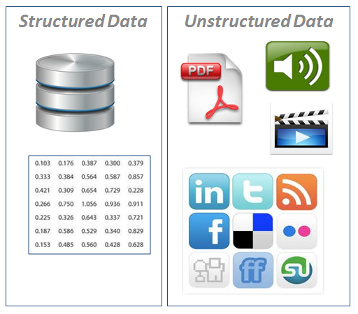
Structured and Unstructured Data

Advantages

Here are some conclusions of why deep learning is advanced comparing to traditional machine learning.

Firstly, deep learning models performs better when dealing with big data. Here is a comparation of deep learning models and classic machine learing models:

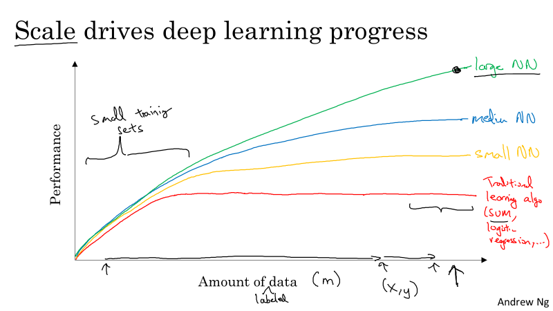
Comparation between deep learning and machine learning

Secondly, thanks to the booming development of hardware and advanced algorithm, computing is much faster than before. Thus, we can implement our idea and know whether it works or not in short time. As a result, we can run the following circle much faster than we image.

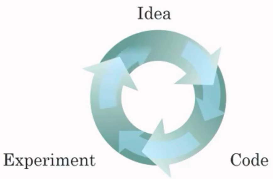
Iteration process

Basic Symbols of the Course

These basic symbols will be used through out the whole specialization.

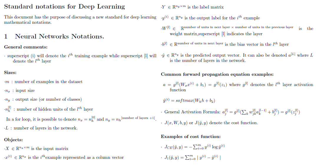
Standard notations

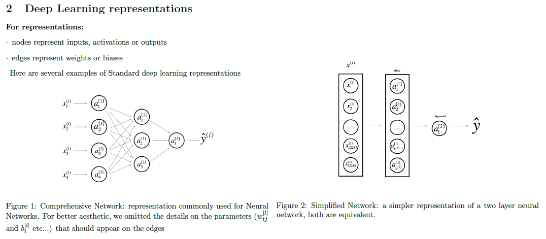
Standard representation

Moreover, in this course, each input x will be stacked into columns and form the input matrix X.

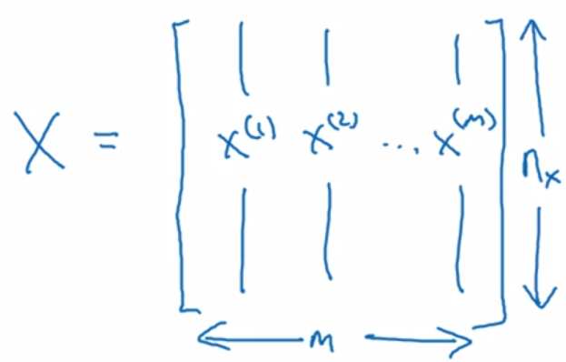
Input X

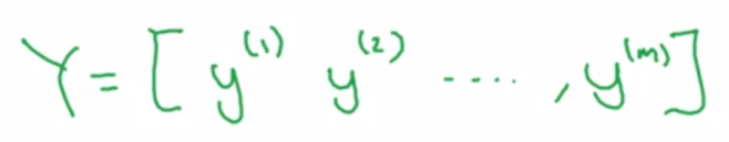
Output y

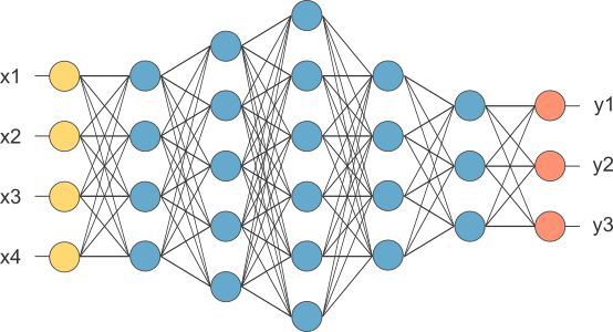
Neural Network

Reviewing the whole course, there are several common concepts between logistic regression and neural network (including both shallow and deep neural network). Thus, I draw conclusions on each concept and then apply them to both logistic regression and neural network.

Logistic Regression and Neural Network

First of all, here are pictures of logistic regression and neural network.

Logistic Regression

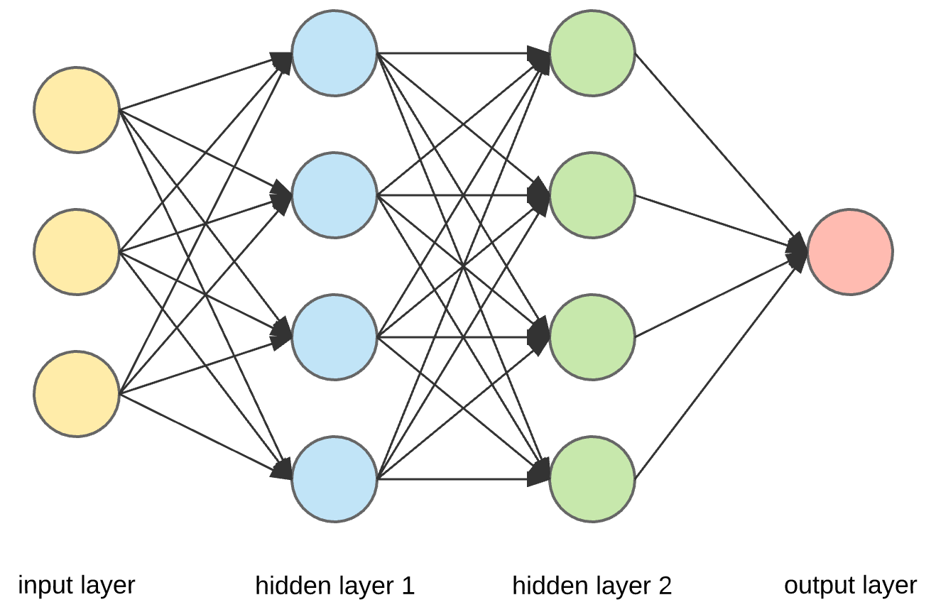
Neural Network

As we can see, logistic regression is also a kind of neural network, which has input layer and output layer and does not have hidden layers, so that it is also called mini neural network. In the following sections, I will write “neural network” to represent logistic regression and neural network and use pictures similar to the second one to represent neural network.

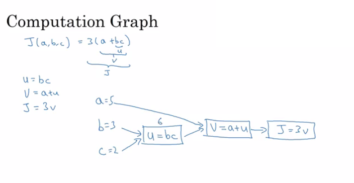
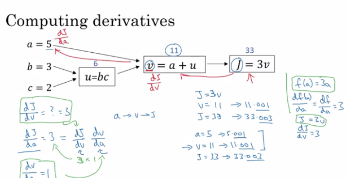
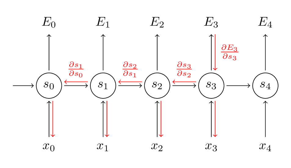
Computation Graph

Computation graph is one of basic concepts in deep learning. By analyzing it, we could understand the whole process of computation process of neural network. The following is the basic computation graph:

In this picture, we can easily understand how $J(a,b,c)=3(a+bc)$ is computed. This process is similar to “Forward Propagation” process which I will say in next section. Moreover, in neural network, $J$ is called cost function. After computing cost function $J$, we need to feed it back to all of our parameters, such as $a$, $b$, $c$ in the picture. This process is called computing derivatives.

By analyzing the comutation graph, we can easily compute all deviatives. According to chain rule, we can compute $\frac{dJ}{da}$ by $\frac{dJ}{dv}\frac{dv}{da}$. So do parameter $b$ and $c$. The whole derivation process is similar to “backward propagation” process in neural network.

Forward Propagation

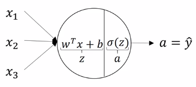
Computation on single neuron

Computation on single neuron

For every single neuron, the computing process is the same as the logistic regression. Logistic regression is basically the combination of linear regression and logistic function such as sigmoid. It has one input layer, x, and one output layer, a or $ \hat{y} $.

The linear regression equation is: $ z = w^Tx+b $
The sigmoid function equation is: $ a = \sigma( z ) $
The combination euquation is:   $ \hat{y} = a = \sigma( w^Tx + b ) $

The whole process on Neural Network

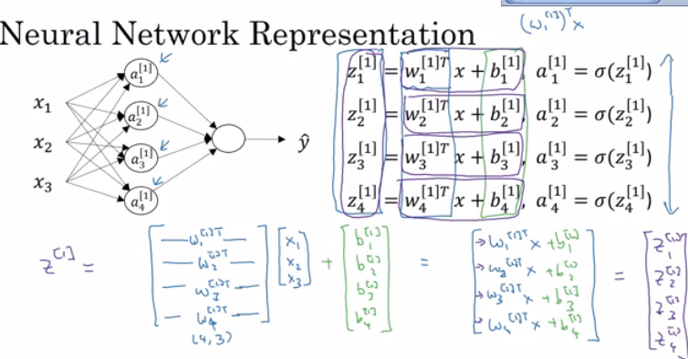
Forward Propagation

This is an example of neural network. Since it only has one hidden layer, it’s also called shallow neural network. The forward propagation process means that we compute the graph from left to the right in this picture.

The whole process when computing the 1^st layer (hidden layer) is as the following:

$$
\begin{align}
Z^{[1]} & = W^{[1]T}X + b^{[1]} \\
A^{[1]} & = \sigma( Z^{[1]} )
\end{align}
$$

In these equations:

• $W^{[1]T}$ is a $4 \times 3$ matrix. It is also written as $W^{[1]}$. Its shape is always $n^{[l]} \times n^{[l - 1]}$.
• $X$ is a $3 \times m$ matrix. Sometimes it is also called $A^{[0]}$.
• $b^{[1]}$ is a $4 \times m$ matrix. Its shape is always $n^{[l]} \times m$.
• $A^{[1]}$ is a $4 \times m$ matrix. Its shape is always $n^{[l]} \times m$.
• $\sigma$ is an element-wise function. It is called activation function.

For each layer, it just repeats what previous layers do until the last layer (output layer).

Cost function

Here is a definition of loss function and cost function.

• Loss function computes a single training example.
• Cost function is the average of the loss function of the whole training set.

In traditional machine learning, we use square root error as loss function, which is $ L = \frac{1}{2}( \hat{y} - y )^2 $. But in this case, we don’t use it since most problems we try to solve are not convex.

Here is the loss function we use:

$$
L( \hat{y}, y ) = -( y \cdot log(\hat{y}) + ( 1 - y ) \cdot log( 1 - \hat{y} ) )
$$

For this loss function:

• if y = 1, then $ L = -y \cdot log(\hat{y}) $ and it will close to 0 when $ \hat{y} $ near 1.
• if y = 0, then $ L = -( 1 - y ) \cdot log( 1 - \hat{y} ) $ and it will close to 0 when $ \hat{y} $ near 0.

Then the cost function is: $$ J( w, b ) = \frac{1}{m}\sum_{i=1}^{m} L( \hat{y}, y ) $$

Backward Propagation

Here, we use gradient descent as our backward propagation method.

Compute Gradients

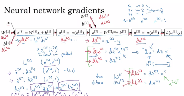
Backward Propagation

As we can see in the picture, it is a simplified computation graph. The neural network is on the right-top, which is almost the same as the neural network we discussing in previous section. Backward Propagation is computing derivatives from the right to the left. By following the backward process, we can get derivatives for all parameters, including $W^{[1]}$, $b^{[1]}$, $W^{[2]}$, $b^{[2]}$.

Here I give a rough derivation example of computing gradients of parameter $W^{[1]}$.

$$
\begin{align}
\frac{\partial L}{\partial Z^{[1]}} & = W^{[2]T}\frac{\partial L}{\partial Z^{[2]}} \cdot {\sigma}^{[1]\prime}(Z^{[1]}) \\
\frac{dL}{dW^{[1]}} & = \frac{\partial L}{\partial Z^{[1]}}\frac{dZ^{[1]}}{dW^{[1]}} \\
& = \frac{\partial L}{\partial Z^{[1]}}A^{[0]T} \\
\frac{dL}{db^{[1]}} & = \frac{\partial L}{\partial Z^{[1]}}\frac{dZ^{[1]}}{db^{[1]}} \\
& = \frac{\partial L}{\partial Z^{[1]}}
\end{align}
$$

It is similar to compute parameters in other layers. In these equations:

• $\frac{dL}{dW^{[1]}}$ has the same shape as $W^{[1]}$. So do other layers.
• $\frac{dL}{db^{[1]}}$ has the same shape as $b^{[1]}$. So do other layers.
• the $\cdot$ in first line is an element-wise product.

Update parameters

After computing gradients, we can update our parameters quickly.

For every parameters (Take layer1 as an example):

$$
\begin{align}
W^{[1]} & = W^{[1]} - \alpha \frac{dL}{dW^{[1]}} \\
b^{[1]} & = b^{[1]} - \alpha \frac{dL}{db^{[1]}}
\end{align}
$$

In above equations, $\alpha$ is called learning rate, which we need to determine before training.

Activation Functions

In previous sections, notation $\sigma$ is used to represent activation function. In neural network, there are five common activation functions: Sigmoid, Tanh, ReLU, Leaky ReLU, and Exponential LU.

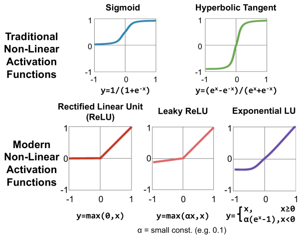
Activation Functions

In the course, Prof. Andrew Ng introduces the first four activation functions.

Here are some experience on choosing those activation functions:

• Sigmoid: It is usually used in output layer to generate results between 0 and 1 when doing binary classification. In other case, you should not use it.
• Tanh: It always works better than sigmoid function since its value is between -1 and 1, so that neural network can learn more information by using it than using sigmoid function.
• ReLU: The most commonly used activation function is ReLU function. If you don’t want to use it, you can choose other ReLU derivatives, such as Leaky ReLU.

Parameters and Hyperparameters

Comparation of shallow and deep neural network

最近跟着老师参加了CWMT评测任务，稍微整理下目前用到的数据清洗相关的工具及使用方法。本人目前操作全在Ubuntu16.04下进行。